The camping trailer case study last month illustrated the difference between solving electrical problems in textbooks versus in the real world. Determining what sources, loads and wiring are there can be a challenge. Wiring diagrams or schematics may not be up-to-date. Loads might be changed out without the facility manager’s or electrical staff’s knowledge. And there are the added effects of multiple sources of electrical energy.
The camping trailer issue didn’t require overly complex troubleshooting, but it did provide additional knowledge about this electrical-system-in-miniature as the process progressed. Owner’s manuals are not written to help the electrician, and you should use online information sources at your own risk. Even feedback from the trailer’s owner can have misconceptions.
Voltage | Current | LOAD Imp | Delta V | Delta I | Source IMP | Ratio | |
120.3 | 7.8 | 15.4 | 0.2 | 0.7 | 0.3 | 54 | |
Typical Stable | 120.1 | 8.5 | 14.1 | ||||
120.2 | 7.6 | 15.8 | 0.1 | 0.9 | 0.1 | 142 | |
119.8 | 9.2 | 13.0 | 0.3 | 0.7 | 0.4 | 30 | |
118.6 | 11.1 | 10.7 | 1.5 | 2.6 | 0.6 | 19 | |
119.5 | 10.2 | 11.7 | 0.6 | 1.7 | 0.4 | 33 | |
120.0 | 8.7 | 13.8 | 0.1 | 0.2 | 0.5 | 28 | |
108.4 | 14.4 | 7.5 | 11.7 | 5.9 | 2.0 | 4 | |
118.6 | 10.9 | 10.9 | 1.5 | 2.4 | 0.6 | 17 | |
121.3 | 6.5 | 18.7 | 1.2 | 2 | 0.6 | 31 | |
Averages | 13.2 | 0.6 |
The trailer did highlight the challenges for a facility using other power sources, such as rooftop solar panels, as well as for an electric utility with multiple distributed energy resources powering the grid. For example, the air conditioner was able to run when shore power was present in the daytime, but at night, it would sometimes trip off the 15A breaker in the building (a garage) providing the shore power. That’s due in part to the reduction in current provided from the nonproducing solar panels, other loads in the trailer including lighting and the independent loads on the 15A circuit, such as a pool filter—more sources of confusion.
In some textbook scenarios, the first step is to combine all the impedances into a single valve. The power source is considered an ideal source, meaning it has no impedance and we would never have sags, swells, transients, etc. In most facilities, the breaker panel has dozens of circuits, which affect what happens to the other voltages and currents. This also applies to the source of the electrical power, where multiple transmission circuits are fed by the nonideal source(s). Those sources feed multiple distribution substations with multiple circuits (some with generators), down to a residential neighborhood with several house services fed from a single pole-mounted transformer.
This makes it seem like it’s impossible to solve power quality problems. That isn’t the case if we focus on the problem at hand and don’t get involved in a legal situation that requires indisputable accuracy in the results published. Instead, we use rules of thumb to help the process along and check that the answers make electrical sense and aren’t bucking to win us a Nobel Prize.
Source impedance
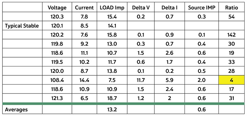
Let’s start with source impedance. From the point-of-common-coupling at a facility service entrance, we can do a simple set of measurements to get an approximation of that value, which is usually in the 0.5- to 2-ohm range. We also initially disregard the complex impedances of the capacitive and inductive elements in the circuits and just focus on the resistive component. The PQ monitor is set up to record voltage and current every minute for a day.
Make a table of valves from the data where the voltage or current seems to change significantly, as well as a dozen or so where those seem stable. Divide the voltage by the current, add up those valves and divide by the number of voltage values you used to get the average load impedance. Now, take one of the voltage values where things seemed stable. Use that to subtract from the voltage values when things changed. Use the current values associated with each of those. Divide the change in voltage (called delta V) by the change in current (delta I). Compute the average of these and you have an approximate source impedance. The load impedance should be 10 times or larger than the source impedance. The table illustrates such a calculation.
This example above uses 120.1V with current of 8.5 as the typical valves for the delta calculations. The ratio of the averages is 22, with a source impedance of less than 1 ohm, meaning the data is most likely accurate enough to be used for analysis processes. When the voltage dropped 10% below the typical, which is often the limit for a voltage sag, the load/source impedance ratio dropped well below the average, as one would expect when the current went significantly up when voltage dropped down.
This is another rule of thumb that we use—directivity. The data points to this sag caused by an event on the load side of the monitoring point, not the source. In other words, it likely wasn’t the utility’s fault.
About The Author

BINGHAM, a contributing editor for power quality, can be reached at 908.499.5321.